Circumventing poor mixing in Bayesian model-based clustering

Summary

Paper: Consensus Clustering for Bayesian Mixture Models

• Aim: Perform inference on Bayesian clustering methods when chains do not converge without reimplementation
• Pros: Easy to use and offers useful inference
• Cons: Inference is no longer Bayesian

Introduction

The first paper of my PhD was entitled “Consensus Clustering for Bayesian Mixture Models” and written with my supervisors Paul and Chris. To overcome the issue of poor mixing that haunts Bayesian clustering, we proposed a heuristic method based on the consensus clustering algorithm of Monti et al. (2003) that appears to enable principled inference without reimplementing the sampler. However, the inference does lose the Bayesian interpretation.

If you have attempted to infer discrete latent structure using a Bayesian method implemented using Markov Chain Monte Carlo (MCMC) methods, then you’ve probably encountered the problem of poor mixing where chains become trapped in different clusterings and stop exploring the parameter space.There is a large body of literature about methods for navigating this problem in a principled fashion (see, e.g., Dahl 2003; Jain and Neal 2004; Bouchard-Côté, Doucet, and Roth 2017; Syed et al. 2022), but these state-of-the-art samplers tend to be time-consuming to implement. In this paper we proposed taking samples from many (relatively) short chains rather than a single long chain. This idea has seen a lot of mileage recently across a few different papers, but where we differ is we surrender our claim of being truly Bayesian. We have to do this as, while it is possibly that our samples are drawn from the target density, they are unlikely to be weighted correctly. However, we found that the expected values from the distributions sampled this way tended to be correct even if the variance might be too large.

Algorithm

The basic method is sketched below:

Consensus clustering for Bayesian methods
Inputs:
  W: the number of chains to run
  D: the number of iterations to run each chain for
  sampler: the MCMC sampler for the method
  priorDraw(): a method of drawing a sample from the prior distribution over the clustering space (this is often integrated into the sampler in practice)
 
Output:
  c: a matrix of sampled partitions

Algorithm:
  for(w in 1:W) {
    # Differentiate the model runs using the random seed
    set.seed(w);
    c_0 <- prior();
    for(r in 1:R) {
      # Sample a new clustering based on the current partition
      c_r <- sampler(c_r);
    }
    # Save the last iteration
    c[w] <- c_r
  }

Obviously one can sample more quantities than just the clustering (as we do in the paper), but I think that clustering works particularly well with short chains. This is because we often care about co-clustering probabilities across sampled partitions rather than any single sample being correct; this means that if there is enough variety across a large number of poor (but better than random) sampled partitions we might still infer the correct structure. For other variables we expect that we need longer chains to have the correct expected value from our sampled distribution. The Multiple Dataset Integration (MDI) example in the paper is a good example of this. MDI is an integrative or multi-view Bayesian clustering method. Signal is shared across datasets to inform clustering in each view and the degree to which information should be shared is also inferred. This is represented by the \(\phi\) parameters in the model. To learn meaningful estimate of \(\phi\) and infer dependent clusterings we need to go much further into the chains then we do for clustering a single dataset. This is because for the information to be shared and how it is shared depends on the global clustering structure emerging. This means that the Markov chains have to reach their target density for consensus clustering to offer a useful inference and the chains are long. This means we lose the massive speed gain that very short chains offer, but we still overcome the multi-modality so often present in the posterior distribution of complex latent structure models. Based on this result we suspect that the method generalises to any Bayesian model, but for this vignette I will only explore clustering of a single dataset.

How to use consensus clustering in practice for Bayesian methods

In this post I want to show how to use consensus clustering. First, let’s generate some data. I generate data with two overlapping clustering structures which emerge in different features (this aspect of the data is sometimes referred to as having two different views of the clustering). This ensures multi-modality is present. The data has 200 samples, 15 variables informing each clustering and 40 noise variables. The first clustering has 4 clusters, the second 9 that are (approximately) nested in the first less resolved clustering.

# For ggplot2 theme and data simulation
suppressPackageStartupMessages(library(mdiHelpR))

# For mixture models
suppressPackageStartupMessages(library(mdir))

suppressPackageStartupMessages(library(magrittr))
suppressPackageStartupMessages(library(patchwork))
suppressPackageStartupMessages(library(tidyr))
suppressPackageStartupMessages(library(ggplot2))
suppressPackageStartupMessages(library(dplyr))

# For the Cranmer-von Mises test
suppressPackageStartupMessages(library(twosamples))

set.seed(1)
setMyTheme()

N <- 200
P <- c(15, 15)
P_n <- 20
delta_mu <- c(0.8, 1.1)
K <- c(9, 4)
pi <- list()
pi[[1]] <- rep(1 / K[1], K[1])
pi[[2]] <- c(2, 4, 4, 1)
pi[[2]] <- pi[[2]] / sum(pi[[2]])

n_views <- 2

my_df <- my_data <- NULL
group_IDs <- matrix(0, nrow = N, ncol = n_views)

for (ii in seq(1, n_views)) {
  .x <- mdir::generateSimulationDataset(K = K[ii],
    N = N,
    P = P[ii],
    delta_mu = delta_mu[ii],
    pi = pi[[ii]],
    P_n = P_n
  )

  .data <- scale(.x$data)
  group_IDs[, ii] <- .x$cluster_IDs

  .df <- .data |>
    as.data.frame()
  .df[[paste0("Group", ii)]] <- .x$cluster_IDs

  if (ii == 1) {
    my_df <- .df
    my_data <- .data
  } else {
    my_df <- cbind(my_df, .df)
    my_data <- cbind(my_data, .data)
  }
}

# annotatedHeatmap(my_data, group_IDs[, 1])
# annotatedHeatmap(my_data, group_IDs[, 2])

# Create the annotation data.frame for the rows
anno_row <- data.frame(
  "View_1" = factor(paste("Cluster", group_IDs[, 1])),
  "View_2" = factor(paste("Cluster", group_IDs[, 2]))
) |>
  magrittr::set_rownames(rownames(my_data))

ann_colours <- list(
  "View_1" = c(ggthemes::colorblind_pal()(8), viridis::viridis(1)),
  "View_2" = ggthemes::colorblind_pal()(4)
)

names(ann_colours$View_1) <- paste("Cluster", seq(1, K[1]))
names(ann_colours$View_2) <- paste("Cluster", seq(1, K[2]))

# Create the heatmap
ph <- pheatmap::pheatmap(my_data,
  color = dataColPal(),
  breaks = defineDataBreaks(my_data, dataColPal(), 0),
  annotation_row = anno_row,
  annotation_colors = ann_colours,
  main = "Generated data annotated by clusterings",
  show_colnames = FALSE,
  show_rownames = FALSE
)

ph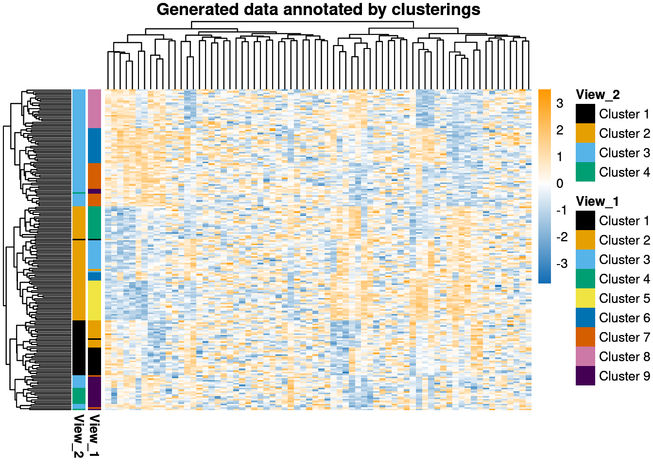

Guessing chain length

To use consensus clustering, we want to have an idea of how long we will need to run the chains for. In this case we run a small number of chains for longer than necessary and the look at trace plots to see when they stopped exploring or the degree of exploration had tapered off significantly.

n_initial_chains <- 9
R_long <- 5000
thin_long <- 50
iterations_initial <- seq(0, R_long, thin_long)

n_samples <- floor(R_long / thin_long) + 1
type <- "G"

psms <- initial_mcmc <- vector("list", n_initial_chains)
likelihood_df <- matrix(0, nrow = n_samples - 1, ncol = n_initial_chains)
colnames(likelihood_df) <- paste0("Chain", seq(1, n_initial_chains))

ari_mat <- concentration_df <- matrix(0, nrow = n_samples, ncol = n_initial_chains)
colnames(ari_mat) <- colnames(concentration_df) <- paste0("Chain", seq(1, n_initial_chains))

ensemble_psm <- matrix(0, nrow = N, ncol = N)

for (ii in seq(1, n_initial_chains)) {
  initial_mcmc[[ii]] <- .mcmc <- callMixtureModel(my_data, R_long, thin_long, type)
  likelihood_df[, ii] <- .mcmc$complete_likelihood[-1]
  concentration_df[, ii] <- .mcmc$mass
  ari_mat[, ii] <- apply(.mcmc$allocations, 1, function(x) {mcclust::arandi(x, .mcmc$allocations[n_samples, ])})
  .psm <- makePSM(initial_mcmc[[ii]]$allocations)
  row.names(.psm) <- colnames(.psm) <- row.names(my_data)
  psms[[ii]] <- .psm
  ensemble_psm <- ensemble_psm + .psm
}

ensemble_psm <- ensemble_psm / n_initial_chains

ari_df <- ari_mat |> 
  as.data.frame() |> 
  mutate(Iteration = iterations_initial) |>
  pivot_longer(-Iteration, names_to = "Chain", values_to = "ARI")

likelihood_df2 <- likelihood_df |>
  as.data.frame() |>
  mutate(Iteration = iterations_initial[-1]) |>
  pivot_longer(-Iteration, names_to = "Chain", values_to = "Complete_log_likelihood")

mass_df <- concentration_df |>
  as.data.frame() |>
  mutate(Iteration = iterations_initial) |>
  pivot_longer(-Iteration, names_to = "Chain", values_to = "Mass")

likelihood_df2 |>
  ggplot(aes(x = Iteration, y = Complete_log_likelihood, group = Chain)) +
  geom_line() +
  ggthemes::scale_color_colorblind()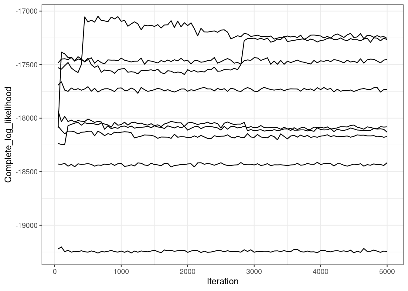

mass_df |>
  ggplot(aes(x = Iteration, y = Mass, group = Chain)) +
  geom_line() +
  ggthemes::scale_color_colorblind()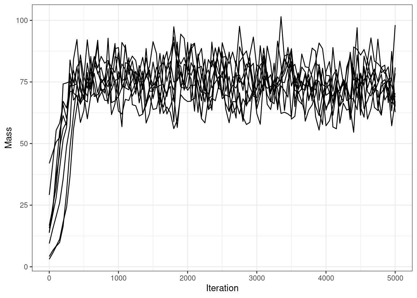

ari_df |> 
  ggplot(aes(x = Iteration, y = ARI, group = Chain)) +
  geom_line() +
  ggthemes::scale_color_colorblind() +
  labs(title = "ARI between rth sampled partition and final sampled partition in each chains")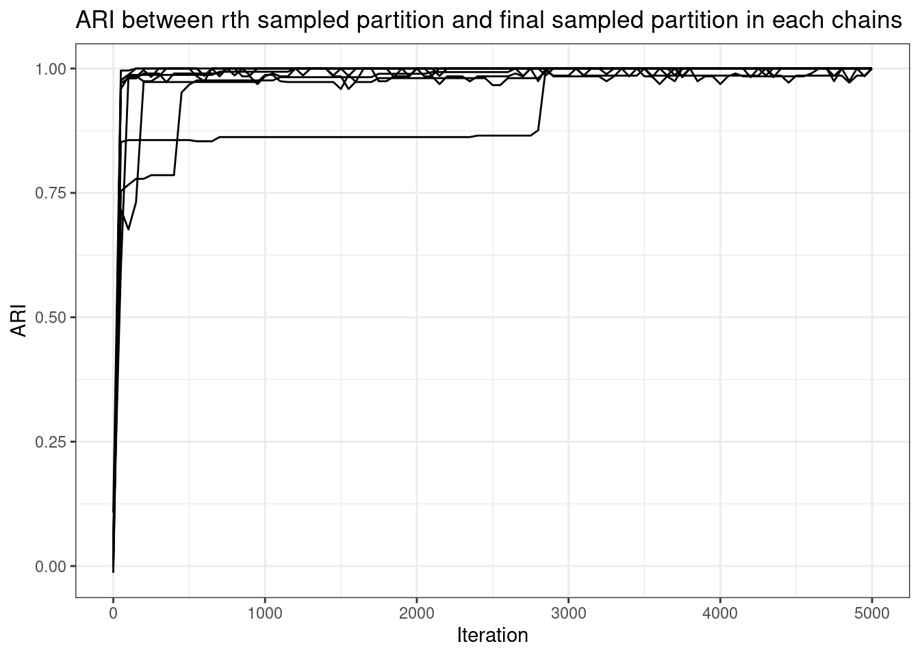

These long chains have stopped exploring new clusterings almost instantly. Two chains do one large change several thousand iterations into the sampler, but all chains find a partition similar to the final sampled partition within 1,000 iteration. The mass parameter takes awhile to converge, but this is sampled via Metropolis-Hastings, so this makes sense.

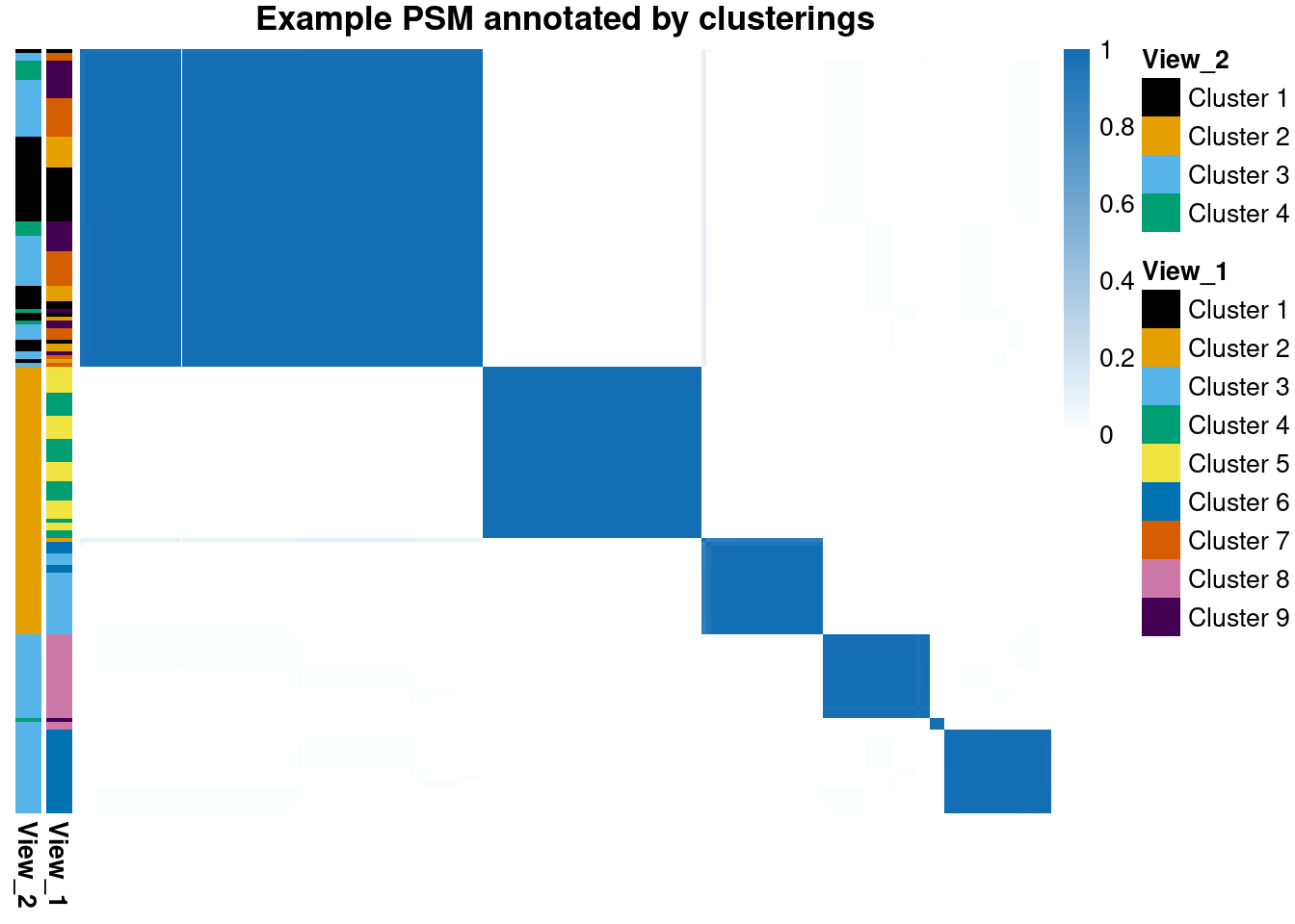
psm <- makePSM(.mcmc$allocations)
row.names(psm) <- colnames(psm) <- row.names(my_data)

# Create the heatmap of the PSM
row_order <- findOrder(psm)
pheatmap::pheatmap(psm[row_order, row_order],
  color = simColPal(),
  breaks = defineBreaks(simColPal(), lb = 0),
  annotation_row = anno_row,
  annotation_colors = ann_colours,
  main = "Example PSM annotated by clusterings",
  show_rownames = FALSE,
  show_colnames = FALSE,
  cluster_rows = FALSE,
  cluster_cols = FALSE
)

psm_df <- prepSimilarityMatricesForGGplot(psms)

psm_df |>
  ggplot(aes(x = x, y = y, fill = Entry)) +
  geom_tile() +
  facet_wrap(~Chain) +
  scale_fill_gradient(
    low = "#FFFFFF",
    high = "#146EB4"
  ) +
  labs(title = "PSMs for initial chains with common ordering") +
  theme(axis.text.x=element_blank(),
    axis.ticks.x=element_blank(),
    axis.text.y=element_blank(),
    axis.ticks.y=element_blank() 
  )

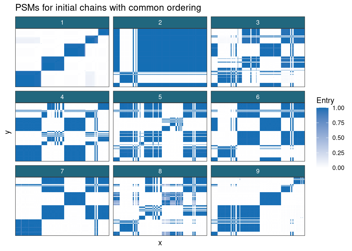
These PSMs also show why nested \(\hat{R}\) and coupling don’t work for clustering. These methods assume that the different chains can eventually reach similar places; this is unlikely to happen in any reasonable length of time in even as low-dimensional an example as this (70 features; hardly low-dimensional in many settings, but that’s one of the joys of ’omics). These PSMs essentially binary, suggesting the same partition is sampled repeatedly; only chains 7 and 8 appear to capture any variety in the clusterings.

Consensus clustering

We now believe that the chains have found whatever structure they are going to find by the 100th iteration, we run an ensemble of chains for an excessive 1,000 iterations.

D_considered <- c(100, 300, 600, 1000)
D <- max(D_considered)
number_depths <- length(D_considered)

W_considered <- c(50, 100, 250, 500)
W <- max(W_considered)
number_chains <- length(W_considered)

models <- expand.grid(D_considered, W_considered)
colnames(models) <- c("Depth", "Width")
n_models <- nrow(models)

thin <- 100
iterations <- seq(0, D, thin)

allocation_list <- consensus_chains <- vector("list", W)

consensus_matrix <- matrix(0, nrow = N, ncol = N)

consensus_matrices <- vector("list", n_models)

allocations <- vector("list", length(D_considered))

# account for saving of 0th iterations
samples_extracted <- (D_considered / thin) + 1

for (ii in seq(1, W)) {
  .mcmc <- callMixtureModel(my_data, D, thin, type)

  for (jj in seq(1, number_depths)) {
    curr_d <- D_considered[jj]
    sample_used <- samples_extracted[jj]

    .alloc <- .mcmc$allocations[sample_used, ]
    .ll <- .mcmc$complete_likelihood[sample_used]
    .mass <- .mcmc$mass[sample_used]

    .lkl_entry <- data.frame(
      "Complete_log_likelihood" = .ll,
      "D" = curr_d,
      "Chain" = ii
    )

    .mass_entry <- data.frame(
      "Mass" = .mass,
      "D" = curr_d,
      "Chain" = ii
    )

    if (ii == 1) {
      allocations[[jj]] <- .alloc
      lkl_df <- .lkl_entry
      mass_df <- .mass_entry
    } else {
      allocations[[jj]] <- rbind(allocations[[jj]], .alloc)
      lkl_df <- rbind(lkl_df, .lkl_entry)
      mass_df <- rbind(mass_df, .mass_entry)
    }
  }
}

cms <- vector("list", n_models)

for (ii in seq(1, number_chains)) {
  curr_w <- W_considered[ii]
  chains_used <- seq(1, curr_w)

  for (jj in seq(1, number_depths)) {
    curr_cm_index <- (ii - 1) * number_depths + jj

    curr_d <- D_considered[jj]
    .cm <- makePSM(allocations[[jj]][chains_used, ])
    row.names(.cm) <- colnames(.cm) <- row.names(my_data)
    cms[[curr_cm_index]] <- .cm
  }
}

cc_lst <- list(
  "CMs" = cms,
  "likelihood_df" = lkl_df,
  "mass_df" = mass_df,
  "allocations" = allocations
)

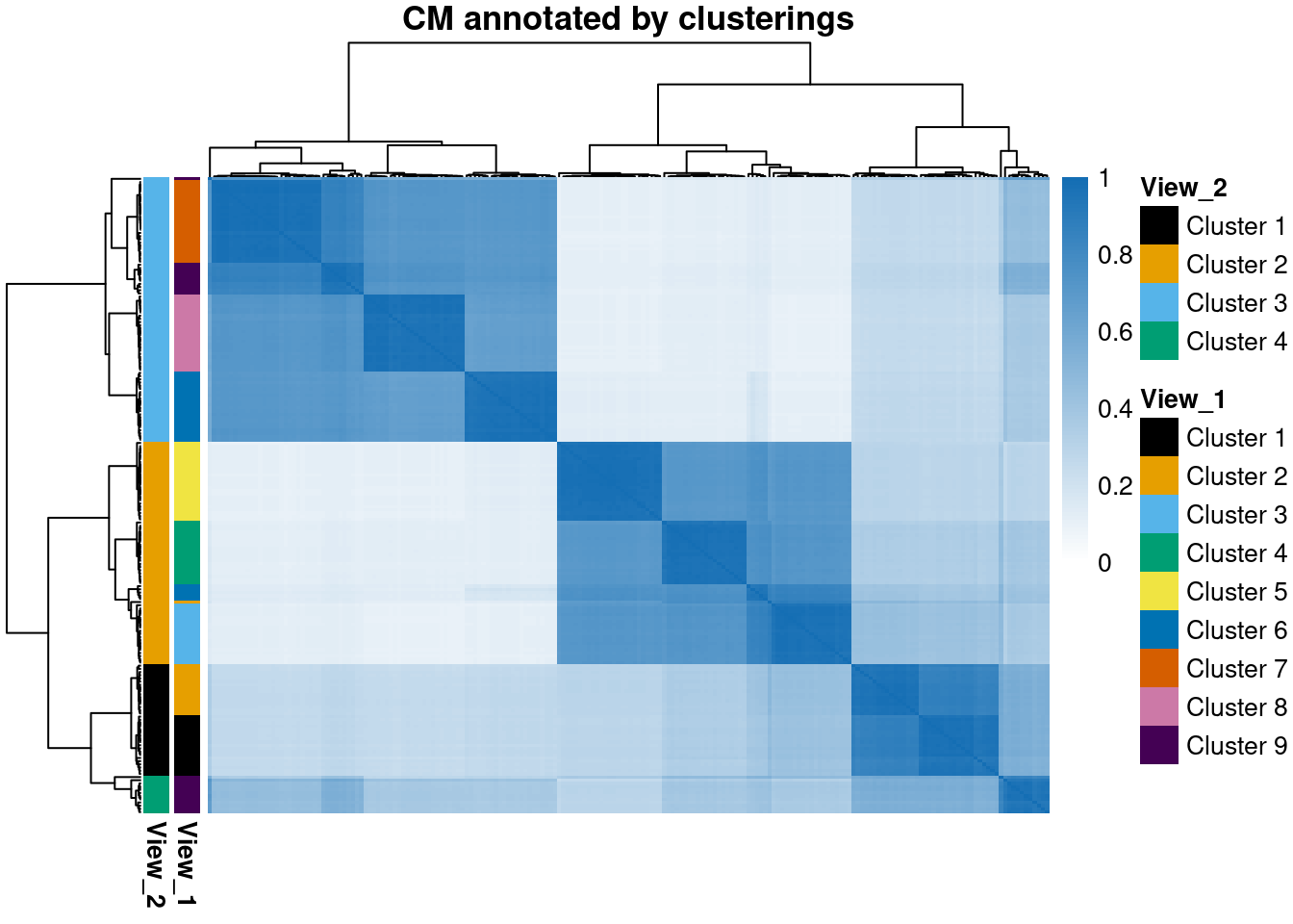
We use the CM from the largest number of chains and deepest sample for some visualisation, annotating by the two different generating clusterings.

pheatmap::pheatmap(cms[[9]],
  color = simColPal(),
  breaks = defineBreaks(simColPal(), lb = 0),
  annotation_row = anno_row,
  annotation_colors = ann_colours,
  main = "CM annotated by clusterings",
  show_colnames = FALSE,
  show_rownames = FALSE
)

Then we consider the trace plots for different samples and numbers of chains.

p_lkl_100 <- lkl_df |>
  filter(Chain < W_considered[1]) |>
  ggplot(aes(x = Complete_log_likelihood, group = D)) +
  geom_density(aes(fill = factor(D)), alpha = 0.4) +
  ggthemes::scale_fill_colorblind() +
  labs(fill = "Chain depth", subtitle = "Complete log-likelihood for 100th sample from each chain")

p_lkl_all <- lkl_df |>
  ggplot(aes(x = Complete_log_likelihood, group = D)) +
  geom_density(aes(fill = factor(D)), alpha = 0.4) +
  ggthemes::scale_fill_colorblind() +
  labs(fill = "Chain depth", subtitle = "Complete log-likelihood for 1,000th sample from each chain")

p_mass_100 <- mass_df |>
  filter(Chain < W_considered[1]) |>
  ggplot(aes(x = Mass, group = D)) +
  geom_density(aes(fill = factor(D)), alpha = 0.4) +
  ggthemes::scale_fill_colorblind() +
  labs(fill = "Chain depth", subtitle = "Mass density for 100th sample from each chain")

p_mass_all <- mass_df |>
  ggplot(aes(x = Mass, group = D)) +
  geom_density(aes(fill = factor(D)), alpha = 0.4) +
  ggthemes::scale_fill_colorblind() +
  labs(fill = "Chain depth", subtitle = "Mass density for 1,000th sample from each chain")

p_lkl_100 / p_lkl_all + plot_annotation(
  title = "Complete log-likelihood for full ensemble and subset of chains",
) + plot_layout(guides = "collect")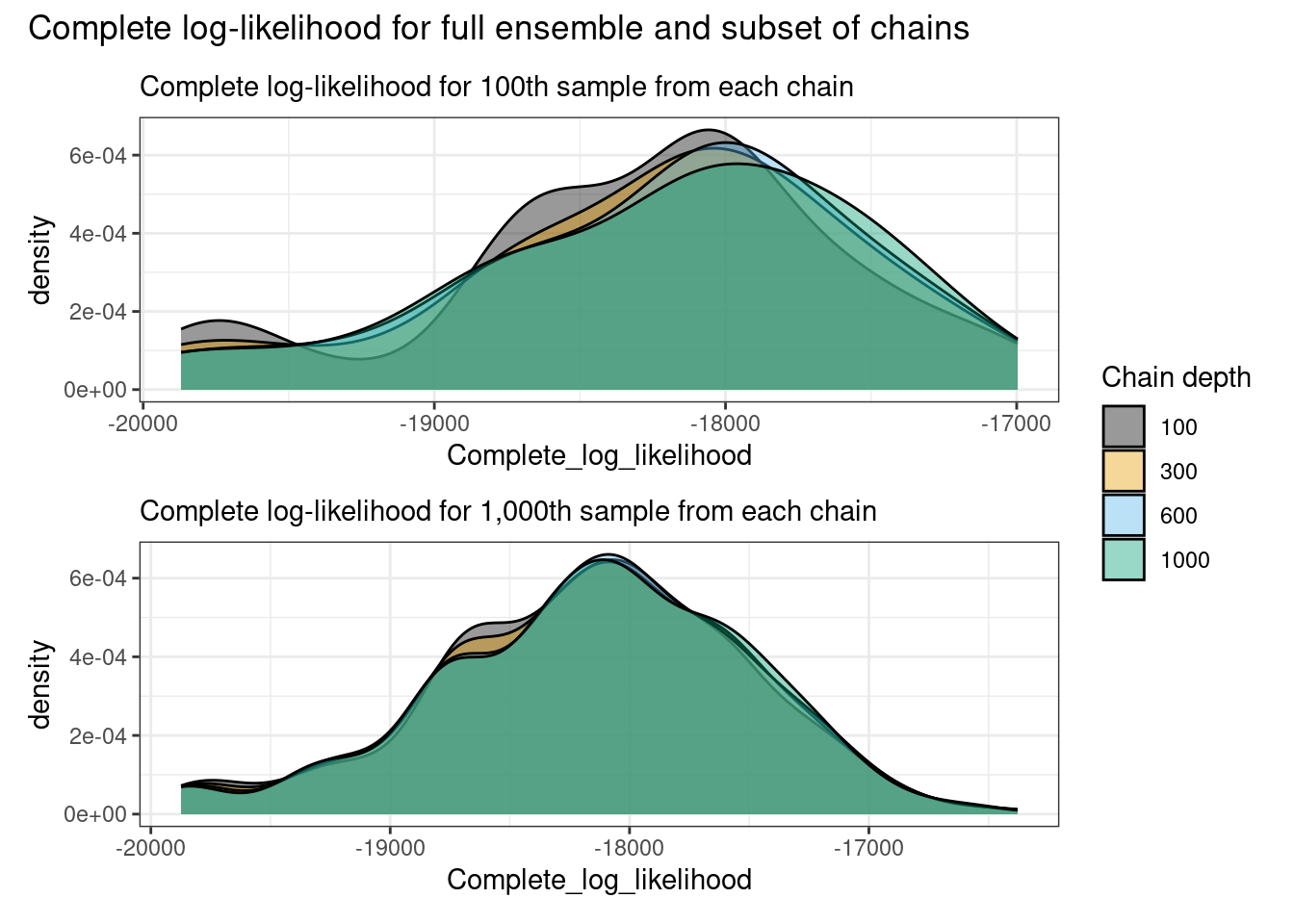

p_mass_100 / p_mass_all + plot_annotation(
  title = "Mass parameter for full ensemble and subset of chains"
) + plot_layout(guides = "collect")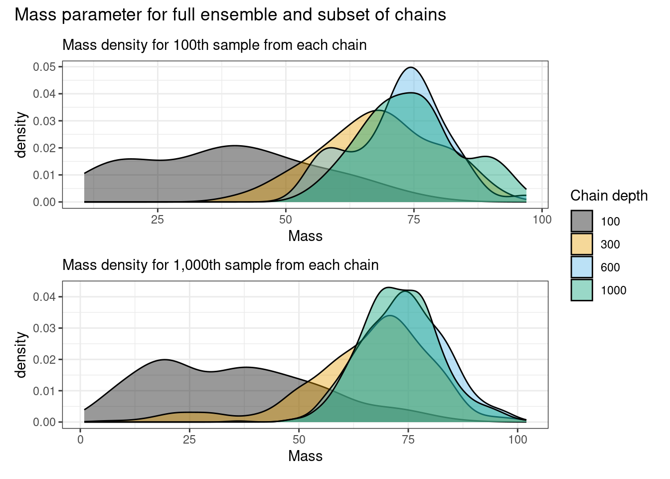

The complete log-likelihoods appear to be stable from the 100th iteration, and sampled mass densities appear to have stabilised by the 500th iteration being slower as it is sampled via Metropolis-Hastings.

cm_df <- prepSimilarityMatricesForGGplot(cms)

cm_df$W <- 1
cm_df$D <- 1

for (ii in seq(1, number_chains)) {
  curr_w <- W_considered[ii]
  # chains_used <- seq(1, curr_w)

  for (jj in seq(1, number_depths)) {
    curr_cm_index <- (ii - 1) * number_depths + jj
    rel_entries <- which(cm_df$Chain == curr_cm_index)

    curr_d <- D_considered[jj]
    cm_df$W[rel_entries] <- curr_w
    cm_df$D[rel_entries] <- curr_d
  }
}


cm_df |>
  mutate(Sample_used = D, Number_chains = W) |>
  ggplot(aes(x = x, y = y, fill = Entry)) +
  geom_tile() +
  facet_grid(Sample_used ~ Number_chains, labeller = label_both) +
  scale_fill_gradient(
    low = "#FFFFFF",
    high = "#146EB4"
  ) +
  theme(axis.text.x=element_blank(),
    axis.ticks.x=element_blank(),
    axis.text.y=element_blank(),
    axis.ticks.y=element_blank() 
  )

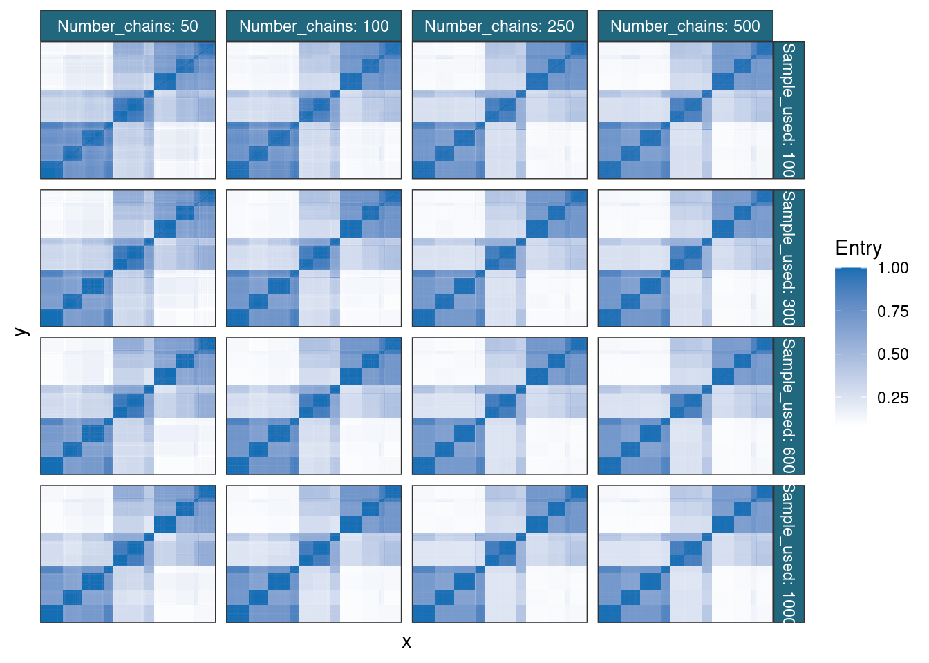
The consensus matrices appear very stable from the smallest and shallowest ensemble, in keeping with the impression from the complete log-likelihoods.

Testing

Testing for convergence in Bayesian inference is difficult. Tests/diagnostics can be split in two categories, within chain and across chain. Within chain stationarity is normally assessed heuristically via trace plots and using the Geweke tests (essentially a t-test between samples at different stages of the chain). For across chains, \(\hat{R}\) dominates. Both of these have shortcomings; for example if a chain explore many modes in the posterior, the Geweke test will suggest discarding it despite this being desirable behaviour in many settings (being a more full depiction of the model uncertainty). Furthermore, when using the Geweke test we want to accept the null hypothesis which is just plain odd. As for \(\hat{R}\), the authors make no claims on how strong a guarantee small values are and this has been the source of much discussion in recent literature with many improvements recommended (see Vats and Knudson 2021; Vehtari et al. 2021; Moins et al. 2022). However, most practitioners still use the original form and the threshold of 1.1.

With this context I would like to argue that the inference from our proposed method can provide a better approximation of the target density than the approach of a single long chain. Our method is more likely to draw samples from the entire support of the posterior, but I suspect it is giving the wrong posterior density to the modes drawn which is the reason I would consider this inference non-Bayesian. However, the logic of convergence can still be applied in considering if we have used a sufficient quantity of chains and if they are of sufficient length. To do this, we would like to assess if the distribution of sampled parameters is not changing for increasing chain length and increasing numbers of chains. My belief is that if the behaviour has stabilised then the chains have reached their stationary distribution and the sample size across chains is sufficiently large to describe the posterior well. We have some disadvantages in that samples across chains are not ordered; however the origin of this property also means that we do not have to worry about auto-correlation across chains and therefore are more robust to multi-modal densities (the big reason to like this approach in my view). Below are two sections, depth tests and width tests that outline my approach to assessing these behaviours. Note that we must tests depth and width separately, much as we test within and across chain convergence separately.

Note that I use t-tests, but we could use something that is more targeted to compare the sampled distributions rather than some summary statistic of them.

Depth tests

Essentially we will follow the logic of Geweke and compare the distribution using early samples to later samples. We differ in that the two sets of samples are collected across many chains, but I think the logic holds. Here we use a Cranmer-von Mises test to test if the sampled distributions of the mass parameter for the clustering and the complete log-likelihood are the same in earlier samples to the same distributions for the final sample from all the chains.

m1 <- mass_df$Mass[mass_df$D == 100]
m2 <- mass_df$Mass[mass_df$D == 300]
m3 <- mass_df$Mass[mass_df$D == 600]
m4 <- mass_df$Mass[mass_df$D == 1000]

l1 <- lkl_df$Complete_log_likelihood[lkl_df$D == 100]
l2 <- lkl_df$Complete_log_likelihood[lkl_df$D == 300]
l3 <- lkl_df$Complete_log_likelihood[lkl_df$D == 600]
l4 <- lkl_df$Complete_log_likelihood[lkl_df$D == 1000]

t_d1_m_1 <- cvm_test(m1, m4)
t_d1_m_2 <- cvm_test(m2, m4)
t_d1_m_3 <- cvm_test(m3, m4)

t_d1_l_1 <- cvm_test(l1, l4)
t_d1_l_2 <- cvm_test(l2, l4)
t_d1_l_3 <- cvm_test(l3, l4)

Width tests

Testing if we are using a sufficient quantity of chains is harder as the chains are not ordered. I believe we can essentially copy the Geweke test again but compare disjoint subsets of samples. For example, take the final sample from a random two fifths of the chains and compare the distribution for these to the distribution from the remaining three fifths and then repeat this multiple times.

frac_used <- 0.4
inds1 <- sample(seq(1, W), size = W * frac_used, replace = FALSE)
inds2 <- sample(seq(1, W), size = W * frac_used, replace = FALSE)
inds3 <- sample(seq(1, W), size = W * frac_used, replace = FALSE)
inds4 <- sample(seq(1, W), size = W * frac_used, replace = FALSE)
inds5 <- sample(seq(1, W), size = W * frac_used, replace = FALSE)

t_w1_m <- cvm_test(m3[inds1], m3[-inds1])
t_w1_l <- cvm_test(l3[inds1], l3[-inds1])

t_w2_m <- cvm_test(m3[inds2], m3[-inds2])
t_w2_l <- cvm_test(l3[inds2], l3[-inds2])

t_w3_m <- cvm_test(m3[inds3], m3[-inds3])
t_w3_l <- cvm_test(l3[inds3], l3[-inds3])

t_w4_m <- cvm_test(m3[inds4], m3[-inds4])
t_w4_l <- cvm_test(l3[inds4], l3[-inds4])

t_w5_m <- cvm_test(m3[inds5], m3[-inds5])
t_w5_l <- cvm_test(l3[inds5], l3[-inds5])

test_df <- data.frame(
  "D" = c(100, 300, 600, D, D, D, D, D),
  "W" = c(W, W, W, 0.2 * W, 0.2 * W, 0.2 * W, 0.2 * W, 0.2 * W),
  "Mass" = c(
    t_d1_m_1[2],
    t_d1_m_2[2],
    t_d1_m_3[2],
    t_w1_m[2],
    t_w2_m[2],
    t_w3_m[2],
    t_w4_m[2],
    t_w5_m[2]
  ),
  "Complete_log_likelihood" = c(
    t_d1_l_1[2],
    t_d1_l_2[2],
    t_d1_l_3[2],
    t_w1_l[2],
    t_w2_l[2],
    t_w3_l[2],
    t_w4_l[2],
    t_w5_l[2]
  )
)

# test_df$Mass <- round(test_df$Mass, 4)
# test_df$Complete_log_likelihood <- round(test_df$Complete_log_likelihood, 4)

Now the p values for the mass parameter and complete log-likelihood t-tests are shown in the below table.

knitr::kable(test_df, caption = "Convergence tests for consensus clustering", digits = 3)

Convergence tests for consensus clustering

D	W	Mass	Complete_log_likelihood
100	500	0.000	0.629
300	500	0.000	0.912
600	500	0.136	1.000
1000	100	0.920	0.570
1000	100	0.554	0.766
1000	100	0.519	0.098
1000	100	0.194	0.025
1000	100	0.769	0.202

The mass is sampled via Metropolis Hastings, so it taking longer to converge than the complete log-likelihood (which is a direct function of the clustering) is not shocking.

Mean abolute difference between consensus matrices

In the paper I recommended using the below kind of plots, but these need more models for assessing as with only three levels of both the iteration and number of chains used we only have two data points for comparisons, so they have some limitations.

mean_abs_diff_df <- makeCMComparisonSummaryDF(cms, models)

mean_abs_diff_df |>
  dplyr::filter(Quantity_varied == "Depth") |>
  ggplot(aes(x = Depth, y = Mean_absolute_difference, color = factor(Width))) +
  geom_line() +
  labs(title = "Assessing stability across cms for increasing chain depth") +
  ggthemes::scale_color_colorblind()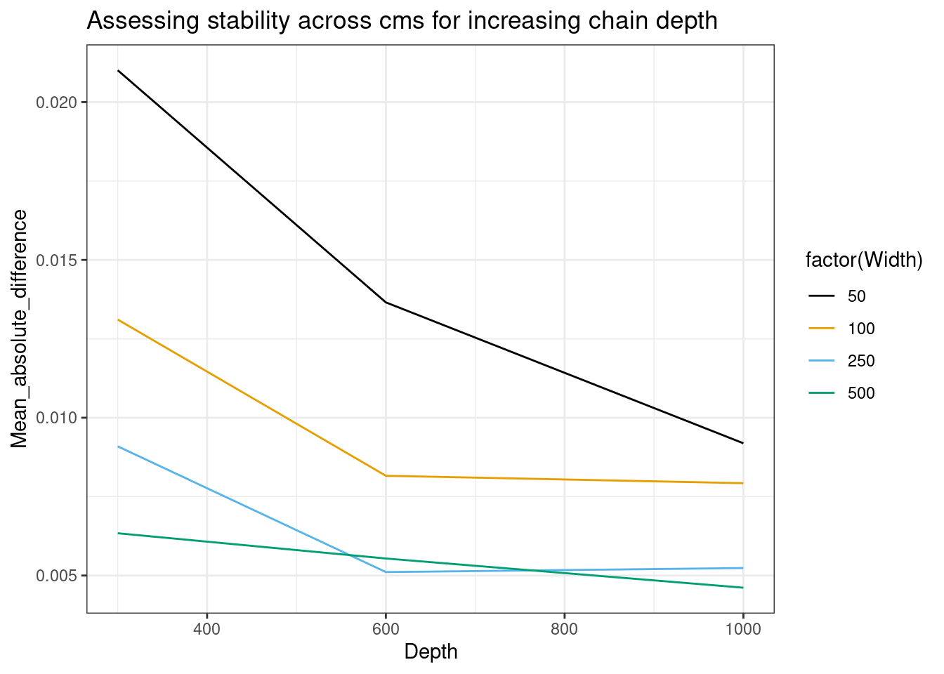

mean_abs_diff_df |>
  dplyr::filter(Quantity_varied == "Width") |>
  ggplot(aes(x = Width, y = Mean_absolute_difference, color = factor(Depth))) +
  geom_line() +
  labs(title = "Assessing stability across cms for increasing numbers of chains") +
  ggthemes::scale_color_colorblind()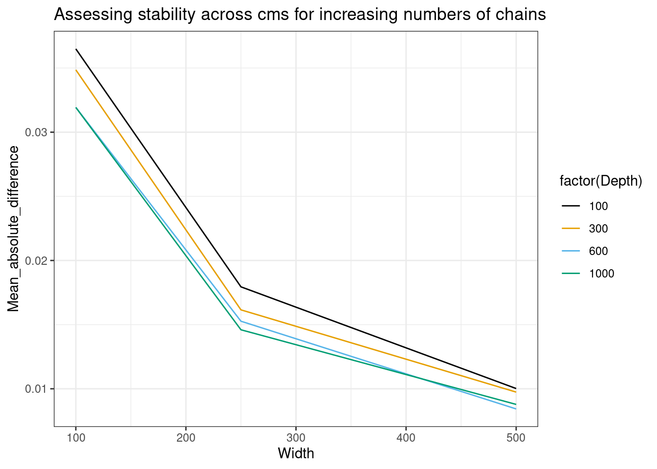

How Bayesian are we?

I am interested in how well the consensus clustering approximates a well-behaved chain. Let’s investigate this in a dataset where mixing will not be an issue. We’ll run a number of chains on a two-dimensional dataset with well separate clusters and compare this to a consensus clustering of the same dataset. In both the short and long chains we will use longer chains than we need.

N_2d <- 200
P_2d <- 2

data_2d <- generateGaussianDataset(cluster_means = c(-2, 2), 
  std_dev = c(1, 1), 
  N = N_2d, 
  P = P_2d, 
  pi = c(0.5, 0.5)
)

D <- 500
W <- 1000

alloc_mat <- matrix(0, nrow = W, ncol = N_2d)

for(w in seq(1, W)) {
  .mcmc <- mdir::callMixtureModel(data_2d$data, D, thin = D, type = "G", K = 50)
  alloc_mat[w, ] <- .mcmc$allocations[2 , ]
}

cm <- mdir::createSimilarityMat(alloc_mat)

n_chains <- 7
R <- 2.5e4
thin <- 25
burn <- 1e4

psms <- list()

for(ii in seq(1, n_chains)) {
  .mcmc <- mdir::callMixtureModel(data_2d$data, R, thin, type = "G", K = 50)
  psms[[ii]] <- mdir::createSimilarityMat(.mcmc$allocations[-seq(1, burn / thin), ])
}

psms[[n_chains + 1]] <- cm

If we compare these PSMs and the consensus matrix we see that they all look very similar.

psm_df <- prepSimilarityMatricesForGGplot(psms)

top_matrices <- psm_df |> 
  filter(Chain %in% c(n_chains, n_chains + 1)) |> 
    mutate(Type = case_when(
      Chain == n_chains ~ paste("Chain", n_chains),
      Chain == n_chains + 1 ~ paste0("CC(", D, ", ", W, ")" )
    )
  )

bottom_matrices <- psm_df |> 
  filter(Chain %in% seq(1, n_chains - 1)) |> 
  mutate(Type = paste0("Chain ", Chain))

p1 <- top_matrices |>
  ggplot(aes(x = x, y = y, fill = Entry)) +
  geom_tile() +
  facet_wrap(~Type) +
  scale_fill_gradient(low = "#FFFFFF", high = "#146EB4") +
  labs(x = "Item", y = "Item", fill = "Coclustering\nproportion") +
  theme(
    axis.text = element_blank(),
    axis.ticks = element_blank(),
    panel.grid = element_blank(),
    axis.title.y = element_text(size = 10.5),
    axis.title.x = element_text(size = 10.5),
    plot.title = element_text(size = 18, face = "bold"),
    plot.subtitle = element_text(size = 14),
    strip.text.x = element_text(size = 10.5),
    legend.text = element_text(size = 10.5)
  )

p2 <- bottom_matrices |>
  ggplot(aes(x = x, y = y, fill = Entry)) +
  geom_tile() +
  facet_wrap(~Type, nrow = 2) +
  scale_fill_gradient(low = "#FFFFFF", high = "#146EB4") +
  labs(x = "Item", y = "Item", fill = "Coclustering\nproportion") +
  theme(
    axis.text = element_blank(),
    axis.ticks = element_blank(),
    panel.grid = element_blank(),
    axis.title.y = element_text(size = 10.5),
    axis.title.x = element_text(size = 10.5),
    plot.title = element_text(size = 18, face = "bold"),
    plot.subtitle = element_text(size = 14),
    strip.text.x = element_text(size = 10.5),
    legend.text = element_text(size = 10.5)
  )
  
p1 / p2 +
  plot_layout(guides = "collect")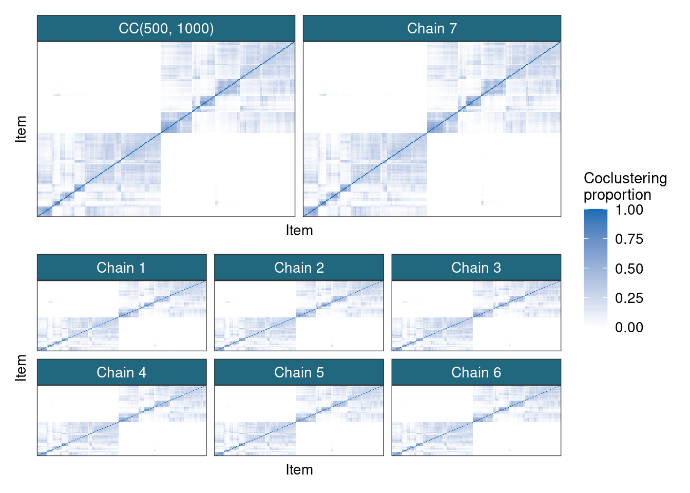

It appears that consensus clustering can describe the posterior distribution quite well, placing an appropriate amount of mass on each potential partition. I don’t think this is sufficient proof to claim that the inference performed using many short chains is truly Bayesian, but it is a close approximation in any of the cases I have looked into. I can imagine settings with poor mixing where using a uniform weighting of MCMC samples ends up placing the wrong mass on the partitions and using some function of the marginal likelihood might be more appropriate, but figuring out the function and the complexity of calculating it might not be worthwhile longterm. Also, I have the impression that uniform weights for averaging across models can be better in terms of prediction or how well it describes unseen data, so even if this heuristic can fail to recover the true posterior, its usefulness might be better than if it had.

References

Bouchard-Côté, Alexandre, Arnaud Doucet, and Andrew Roth. 2017. “Particle Gibbs Split-Merge Sampling for Bayesian Inference in Mixture Models.” Journal of Machine Learning Research 18 (28).

Dahl, David B. 2003. “An Improved Merge-Split Sampler for Conjugate Dirichlet Process Mixture Models.” Technical R Eport 1: 086.

Jain, Sonia, and Radford M Neal. 2004. “A Split-Merge Markov Chain Monte Carlo Procedure for the Dirichlet Process Mixture Model.” Journal of Computational and Graphical Statistics 13 (1): 158–82. https://doi.org/10.1198/1061860043001.

Moins, Théo, Julyan Arbel, Anne Dutfoy, and Stéphane Girard. 2022. “On the Use of a Local \(\hat{R}\) to Improve MCMC Convergence Diagnostic.” arXiv. https://doi.org/10.48550/ARXIV.2205.06694.

Monti, Stefano, Pablo Tamayo, Jill Mesirov, and Todd Golub. 2003. “Consensus Clustering: A Resampling-Based Method for Class Discovery and Visualization of Gene Expression Microarray Data.” Machine Learning 52 (1): 91–118. https://doi.org/10.1023/A:1023949509487.

Syed, Saifuddin, Alexandre Bouchard-Côté, George Deligiannidis, and Arnaud Doucet. 2022. “Non-Reversible Parallel Tempering: A Scalable Highly Parallel MCMC Scheme.” Journal of the Royal Statistical Society: Series B (Statistical Methodology) 84 (2): 321–50. https://doi.org/https://doi.org/10.1111/rssb.12464.

Vats, Dootika, and Christina Knudson. 2021. “Revisiting the Gelman–Rubin Diagnostic.” Statistical Science 36 (4): 518–29. https://doi.org/10.1214/20-STS812.

Vehtari, Aki, Andrew Gelman, Daniel Simpson, Bob Carpenter, and Paul-Christian Bürkner. 2021. “Rank-Normalization, Folding, and Localization: An Improved \(\widehat{R}\) for Assessing Convergence of MCMC (with Discussion).” Bayesian Analysis 16 (2): 667–718. https://doi.org/10.1214/20-BA1221.

Reuse

https://creativecommons.org/licenses/by/4.0/

Citation

BibTeX citation:

@online{coleman,
  author = {Stephen Coleman},
  title = {Circumventing Poor Mixing in {Bayesian} Model-Based
    Clustering},
  url = {https://github.com/stcolema/stcolema.github.io/posts/consensusClustering/consensus_clustering.html},
  langid = {en}
}

For attribution, please cite this work as:

Stephen Coleman. n.d. “Circumventing Poor Mixing in Bayesian Model-Based Clustering.” https://github.com/stcolema/stcolema.github.io/posts/consensusClustering/consensus_clustering.html.