This vignette introduces the mdir R package. This package offers software for Bayesian model based clustering and the Multiple Dataset Integration model for multi-omics analysis. It uses the C++17 parallel policies and thus is unavailable on MAC OS and Debian systems when used with the default C++ compilers.
Model
Multiple Dataset Integration (MDI), is a multi-omics method proposed by Kirk et. al (2012) that extends the Bayesian mixture model to jointly model \(M\) datasets. We introduce the mixture model and then MDI before outlining how to use the mdir package.
Mixture models
Let \(X=(X_1, \ldots, X_N)\) be the observed data, with \(X_n = [X_{n, 1}, \ldots, X_{n,P}]^\top\) for each item being considered, where each observation has \(P\) variables. We wish to model the data using a mixture of densities: \[\begin{align}
p(X_n | \theta = \{\theta_1, \ldots, \theta_K\}, \pi) &= \sum_{k=1}^K \pi_k f(X_n | \theta_k)
\end{align}\] independently for each \(n = 1, \ldots, N\). Here, \(f(\cdot)\) is a probability density function such as the Gaussian density function or the categorical density function, and each component has its own weight, \(\pi_k\), and set of parameters, \(\theta_k\). The component weights are restricted to the unit simplex, i.e., \(\sum_{k=1}^K \pi_k = 1\). To capture the discrete structure in the data, we introduce an allocation variable, \(c=[c_1, \ldots, c_N]^\top, c_n \in [1, K] \subset \mathbb{N}\), to indicate which component a sample was drawn from, introducing conditional independence between the components, \[\begin{align}
p(c_n = k) &= \pi_k, \\
p(X_n | c_n = k, \theta_k) &= f(X_n | \theta_k).
\end{align}\] The joint model can then be written \[\begin{align}
p(X, c, K, \pi, \theta) &= p(X | c, \pi, K, \theta) p(\theta | c, \pi, K) p(c | \pi, K) p(\pi | K) p(K).
\end{align}\] We assume conditional independence between certain parameters such that the model reduces to \[\begin{align}
p(X, c, \theta, \pi, K) &= p(\pi | K) p(\theta | K) p(K) \prod_{n=1}^N p(X_n | c_n, \theta_{c_n}) p (c_n | \pi). \label{eqn:jointMixModel}
\end{align}\] In terms of the hierarchical model this is: \[\begin{align}
X_n | c_n, \theta &\sim F(\theta_{c_n}), \\
c_n | \pi &\sim \text{Multinomial}(\pi_1, \ldots, \pi_K), \\
\pi_1, \ldots, \pi_K &\sim \text{Dirichlet}(\alpha / K, \ldots, \alpha / K), \\
\theta_k &\sim G^{(0)},
\end{align}\] where \(F\) is the appropriate distribution (e.g., Gaussian, Categorical, etc.) and \(G^{(0)}\) is some prior over the component parameters.
MDI
MDI is a Bayesian integrative or multi-modal clustering method. Signal sharing is defined by the prior on the cluster label of the \(n^{th}\) observation in the \(M\) modalities: \[\begin{align}
p(c_n^{(1)}, \ldots, c_n^{(M)} | \cdot) &= \prod_{m=1}^M \gamma^{(m)}_{c_n^{(m)}} \prod_{m = 1}^{M-1} \prod_{l = m + 1}^M (1 + \phi_{(m, l)} \mathbb{I} (c_n^{(m)} = c_n^{(l)})),
\end{align}\] where \(c_n^{(m)}\) is the label of the \(n^{th}\) observation in the \(m^{th}\) modality, \(\gamma^{(m)}_{k}\) is the weight of the \(k^{th}\) cluster in the \(m^{th}\) modality, \(\phi_{(m, l)}\) is the similarity between the clusterings of the \(m^{th}\) and \(l^{th}\) modalities and \(\mathbb{I}(x)\) is the indicator function returning 1 if \(x\) is true and 0 otherwise. Attractively, \(\phi_{(m, l)}\) is inferred from the data and if there is no shared signal it will tend towards 0 giving us no dependency between these modalities. Thus each dataset will have independent clusters.
Data generation
To showcase the MDI method, we generate three datasets with correlated clustering structures. To do this we load the appropriate packages and write some functions to ensure our data do have related generating structure.
library(mdir)library(mdiHelpR)
Attaching package: 'mdiHelpR'
The following objects are masked from 'package:mdir':

    createSimilarityMat, findOrder, generateGaussianDataset,
    generateSimulationDataset, runMDI
The following object is masked from 'package:methods':

    show
library(batchmix)
Attaching package: 'batchmix'
The following object is masked from 'package:mdiHelpR':

    createSimilarityMat
The following objects are masked from 'package:mdir':

    calcAllocProb, createSimilarityMat, gammaLogLikelihood,
    generateInitialLabels, getLikelihood, invGammaLogLikelihood,
    invWishartLogLikelihood, plotLikelihoods,
    predictFromMultipleChains, processMCMCChain, processMCMCChains,
    runMCMCChains, wishartLogLikelihood
library(magrittr)library(mcclust)
Loading required package: lpSolve
RcppParallel::setThreadOptions()setMyTheme()set.seed(1)generateGaussianView <-function(cluster_means, std_devs, N, P, labels,row_names =paste0("Person_", 1:n),col_names =paste0("Gene_", 1:p)) { gen_data <-matrix(0, N, P)for (ii inseq(1, P)) { reordered_cluster_means <-sample(cluster_means) reordered_std_devs <-sample(std_devs)# Draw n points from the K univariate Gaussians defined by the permuted means.for (jj inseq(1, N)) { .mu <- reordered_cluster_means[labels[jj]] .sd <- reordered_std_devs[labels[jj]]# print(labels[jj])# print(.mu)# print(.sd) gen_data[jj, ii] <-rnorm(1,mean = .mu,sd = .sd ) } } gen_data}generateCategoricalView <-function(probs, N, P, labels,row_names =paste0("Person_", 1:n),col_names =paste0("Gene_", 1:p)) { gen_data <-matrix(0, N, P)for (ii inseq(1, P)) { reordered_probs <-sample(probs)# Draw n points from the K univariate Gaussians defined by the permuted means.for (jj inseq(1, N)) { .p <- reordered_probs[labels[jj]] gen_data[jj, ii] <-sample(c(0, 1), 1, prob =c(1- .p, .p)) } } gen_data}generateViewGivenStructure <-function(generating_structure, frac_present, P, K, class_weights, type, params) { N <-length(generating_structure) labels_transferred <-sample(c(0, 1), N, replace =TRUE, prob =c(1- frac_present, frac_present)) labels_transferred_ind <-which(labels_transferred ==1) N_transferred <-sum(labels_transferred) N_new <- N - N_transferred identical_view <- N_new == N K_ind <-seq(1, K) labels <-rep(0, N) labels[labels_transferred_ind] <- generating_structure[labels_transferred_ind]if (!identical_view) { new_labels <-sample(K_ind, N - N_transferred, replace =TRUE, prob = class_weights) labels[-labels_transferred_ind] <- new_labels } gaussian <- type =="G" categorical <- type =="C"if (gaussian) { means <- params$means std_devs <- params$std_devs gen_data <-generateGaussianView(means, std_devs, N, P, labels) }if (categorical) { probs <- params$probs gen_data <-generateCategoricalView(probs, N, P, labels) }row.names(gen_data) <-names(generating_structure)list(gen_data = gen_data,labels = labels )}
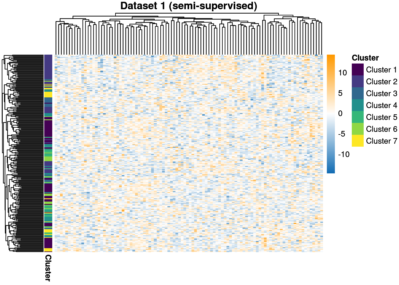
We generate three datasets (sometimes called modalities or views) containing 250 individuals. Our first dataset is generated from 7 classes and contains 400 features. To complicate the matter, we use the data generation method from the batchmix package. This models batch noise and variance using (essentially) a mixture-of-mixtures. Thus our model is misspecified in this dataset, as we will use a Gaussian to describe each class rather then a mixture of multivariate t densities, which is the generating model.
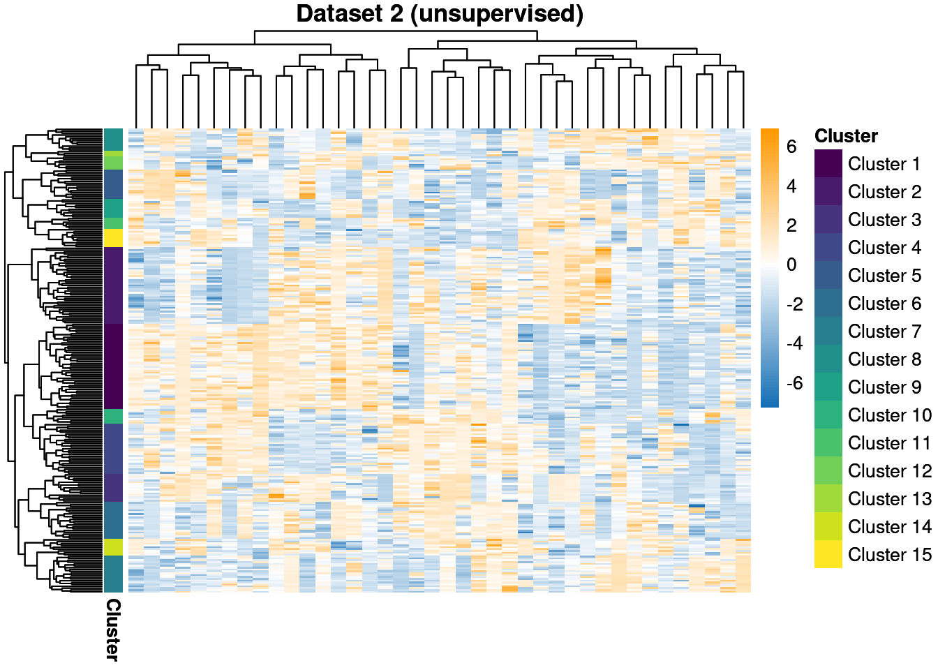
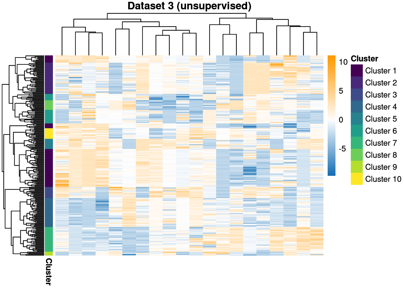
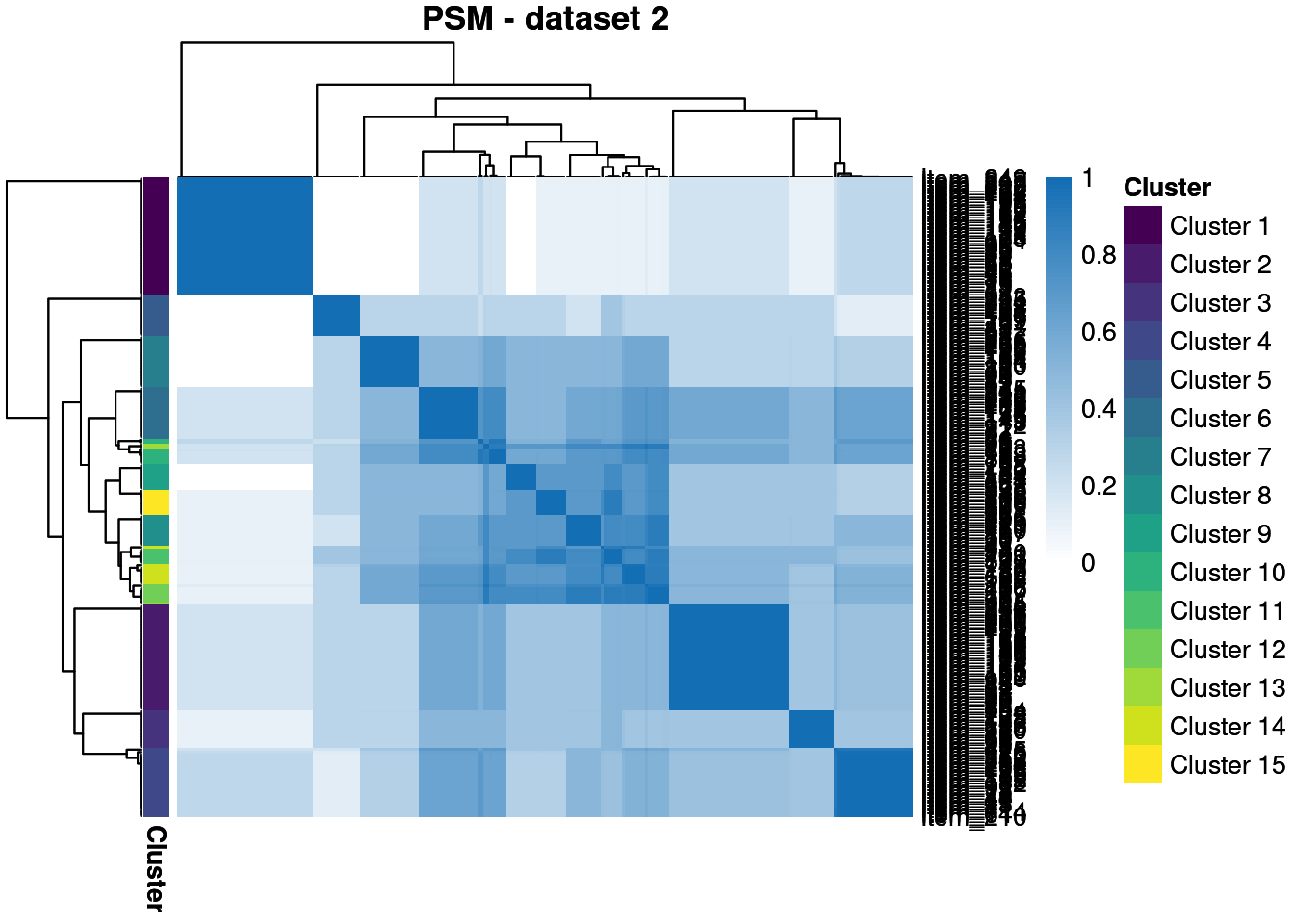
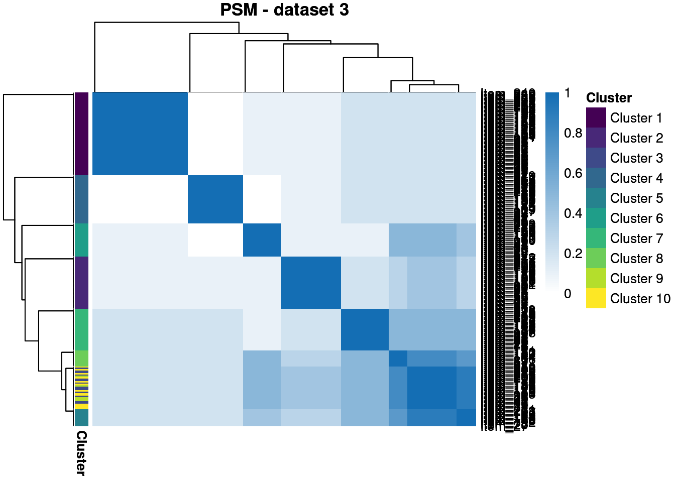
Our second and third datasets are smaller with 25 and 20 features respectively. They also contain more clusters, with 15 and 10 generating clusters compared to the 7 in the first dataset. These data will be modelled with no observed labels, i.e. they are unsupervised, whereas the first dataset has 20% of the labels observed and is semi-supervised within the MDI framework.
We run 5 chains of MDI for 15,000 iterations. In the second and third datasets we use an excessive number of components, similar to an overfitted mixture model, to approximate a Dirichlet process and infer the number of clusters present.
We use a Gaussian density to model each class/cluster.
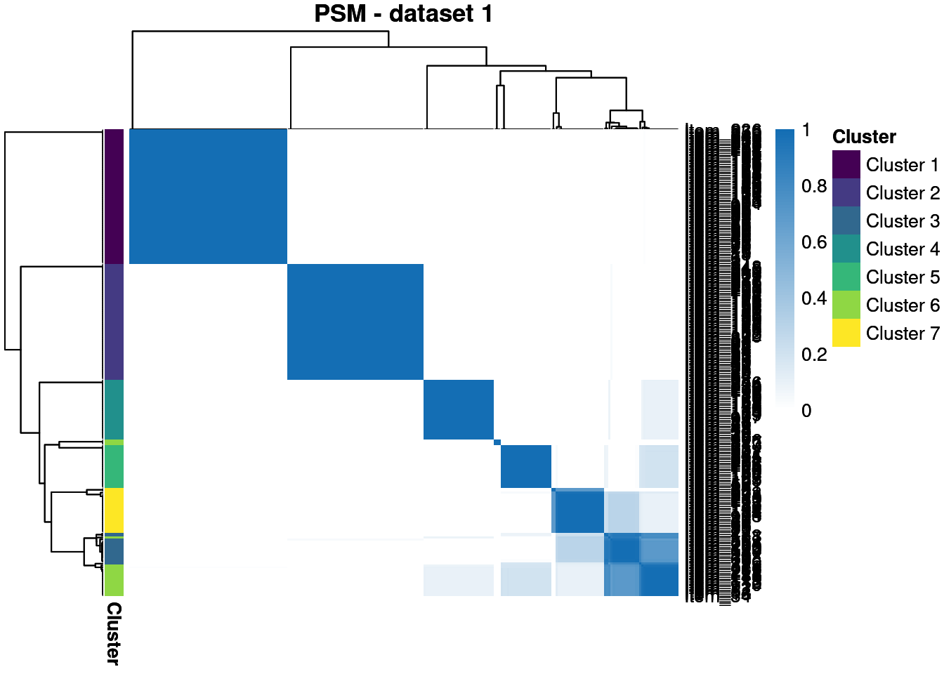
We throw away for the first 20% of samples to remove the warm-up bias and construct posterior similarity matrices to show how well the method captured the structure and the uncertainty about this.
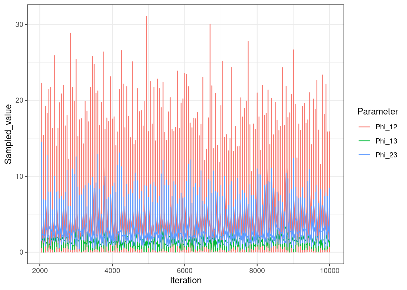
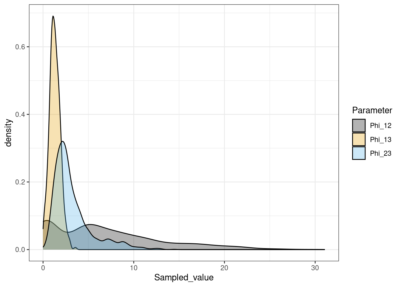
We also look at the \(\phi\) vector. In MDI this reflects how much information is shared between each pair of views and is also inferred from the data.
We see that \(\phi_{1,2}\) is the largest, showing that the most information is shared between these views, matching higher similarity in the generating structures.
Finally, how well do our point estimates align with the true structure?
# Only use the unobserved labels in the first datset for fair comparisontest_inds <-which(fixed[, 1] ==0)ari_1 <-arandi(mcmc_semi$pred[[1]][test_inds], gen_data$group_IDs[test_inds])ari_2 <-arandi(mcmc_semi$pred[[2]], gen_view_2$labels)ari_3 <-arandi(mcmc_semi$pred[[3]], gen_view_3$labels)ari_df <-data.frame("Dataset"=c(1, 2, 3), "ARI"=c(ari_1, ari_2, ari_3))knitr::kable(ari_df, digits =3)
Dataset
ARI
1
0.962
2
0.345
3
0.686
round(mcmc_semi$Time, 1)
Time difference of 26.2 mins
We see that in the semi-supervised dataset we uncover the generating structure with great success, but the point estimates in the other datasets are less good. However, the PSMs show that we have uncovered the true clusterings with some success, even if there is high uncertainty about this.
It takes about 26 minutes to run the ten chains for 10,000 iterations each on the three datasets on the laptop I have built this vignette on.